Car rental problem

I'd like to present to you the problem I stumbled upon in the R. Sutton and A. Barto book about reinforcement learning and really liked. You manage two locations for car rental and try to maximize your profit by moving available cars around locations. It can be seen as a very close model to the real-world situation. It is also very convenient to show how to approach and solve such problems in terms of the RL.

Original text:

The notebook for the article is available at .

Mathematical formulation

Let's rewrite the problem in RL terms. Then we will use the value iteration to find optimal value function \(V(s)\) and policy \(\pi(s)\).

Our state here is \(s = (n_0, n_1)\) for cars at location 0 and location 1 at the end of some day. Then we take action \(a \in -5, \ldots, 5\) and at the start of the next day we have \((n_0 - a, n_1 + a)\). Note that some actions are pointless or incorrect for some states, e.g. \(s = (2, 1)\) and \(a = 5\). For these cases we will add a terminal dummy state with zero reward. All pointless/incorrect \((s, a)\) pairs will transition to it with probability one.

After, we have some realization of poisson rental requests \((\text{req}_0, \text{req}_1)\) and returns \((\text{ret}_0, \text{ret}_1)\) for each location. Note that the reasonable values for rental requests are \(0, \ldots, n_0 - a\) and \(0, \ldots, n_1 + a\). That's why we can truncate poisson random variables to their maximum values. The probability of all values greater adds to the probability of the maximum value. Having the request values, the reasonable values for returns are \(0, \ldots, 20 - (n_0 - a - \text{req}_0)\) and \(0, \ldots, 20 - (n_1 + a - \text{ret}_1)\). So returns are truncated as well. The final state is $s' = (n_0 - a - \text{req}_0 + \text{ret}_0, n_1 + a - \text{req}_1 + \text{ret}_1) $. To compute probability of such a transition we use independence of the requests and returns so their mutual probability is a product of individual probabilities. Overall, we can compute \(p(s' | s, a)\) by fixing \((s, a)\) and iterating over reasonable realizations of \((\text{req}_0, \text{req}_1)\) and \((\text{ret}_0, \text{ret}_1)\), adding \(\mathbb{P}(\text{req}_0, \text{req}_1, \text{ret}_0, \text{ret}_1)\) to corresponding \(s'\).

Reward \(r(s, a, s')\) here is a random variable for fixed arguments because it depends on the random requests and returns. To use it in the dynamical programming we need to average it over valid \((\text{req}_0, \text{req}_1, \text{ret}_0, \text{ret}_1)\) for given \((s, a, s')\). We can do it during the same iteration when computing \(p(s' | s, a)\). We init \(r(s, a, s')\) with zeros. Then, for fixed \((s, a)\) and realization of the requests and returns the reward is uniquely determined. We multiply it with the probabilty of such realization and add to \(r(s, a, s')\). After all iterations we have completed \(p(s' | s, a)\) and averaged \(r(s, a, s')\) but unnormed. The normalization constant for averaging is exactly \(p(s' | s, a)\).

To compute optimal value function and policy we will use value iteration algorithm which basically solves the following equation iteratively:

The optimal policy is then obtained as

Implementation details

We init five dimensional tensors for probability and reward:

1
2
3
4
5
6
7
8
9

  n_actions = 2 * max_cars_moved + 1
  # dims go (n0, n1, a, n0', n1')
  reward_t = np.zeros(
      [max_cars_location + 1] * 2 + [n_actions] + [max_cars_location + 1] * 2
  )
  # init p(s' | s, a), dims go (n0, n1, a, n0', n1')
  prob_t = np.zeros(
      [max_cars_location + 1] * 2 + [n_actions] + [max_cars_location + 1] * 2
  )

We then iterate over all starting states and actions, then over all reasonable rental requests. In the inner-most cycle the reasonable return requests are easily determined as well as their probabilities.

 1
 2
 3
 4
 5
 6
 7
 8
 9
10
11
12
13
14
15
16
17
18

  for (n0, n1) in product(
    range(0, conf.max_cars_location + 1), 
    range(0, conf.max_cars_location + 1)
  ):
    for cars_moved in range(-conf.max_cars_moved, conf.max_cars_moved + 1):
      # num of cars at the start of the day
      n0_start = n0 - cars_moved
      n1_start = n1 + cars_moved
      for (req0, req1) in product(range(0, n0_start + 1), range(0, n1_start + 1)):
        # cars left after requests
        cars_left0 = n0_start - req0
        cars_left1 = n1_start - req1
        # maximum number of cars that can be returned
        max_returns0 = conf.max_cars_location - cars_left0
        max_returns1 = conf.max_cars_location - cars_left1
        # probabilities for possible requests
        prob_req0 = truncate_distr_probs(lambda_req_0, n0_start)
        prob_req1 = truncate_distr_probs(lambda_req_0, n1_start)

We also compute probabilities of the truncated poisson variables for the retuns. Their mutual probability can be computed via np.outer. The reward is constant in the inner-most loop because it depends only on the action and the rental requests. Finally, we add up probaility and mean reward to all possible states we transition to under current realizations of the poisson variables.

 1
 2
 3
 4
 5
 6
 7
 8
 9
10
11
12
13
14
15
16
17
18

  # probabilities for possible returns
  prob_ret0 = truncate_distr_probs(lambda_ret_0, max_returns0)
  prob_ret1 = truncate_distr_probs(lambda_ret_1, max_returns1)
  # compute mutual probabilites for returns
  prob_ret = np.outer(prob_ret0, prob_ret1)
  # reward for current realization
  reward = (req0 + req1) * rent_price - \
                  np.abs(cars_moved) * conf.move_price

  # add a fraction to the expected reward for (s, a) = fixed
  # and s' - varied
  reward_t[
      n0, n1, act_indx, cars_left0:, cars_left1:
  ] += reward * (prob_req0[req0] * prob_req1[req1] * prob_ret)
  # add a fraction to the probability for (s, a) = fixed and s' - varied
  prob_t[
      n0, n1, act_indx, cars_left0:, cars_left1:
  ] += prob_req0[req0] * prob_req1[req1] * prob_ret

After all loops we normalize average reward as was said:

1

reward_t[prob_t != 0.] = reward_t[prob_t != 0.] / prob_t[prob_t != 0.]

In the value iteration we flatten state dims so our tensors will have three dimensions \((s, a, s')\). It is convenient to use np.einsum to compute mean values over probability transition function:

from scipy import linalg


def value_iteration(
    reward_t: np.ndarray,
    prob_t: np.ndarray,
    gamma: float,
    v0: np.ndarray,
    tol: float = 1e-3,
    max_steps: int = 1000
) -> np.ndarray:
    # compute avereged over s' reward r(s, a, s')
    reward_expect = np.einsum(
        "iaj,iaj->ia",
        prob_t, reward_t
    )
    v_prev = v0
    for _ in range(max_steps):
        v_expect = np.einsum(
            "iaj,j->ia",
            prob_t, v_prev
        )
        v = np.max(reward_expect + gamma * v_expect, axis=-1)

        delta = linalg.norm(v - v_prev, np.inf)
        if delta < tol:
            break
        v_prev = v

    return v

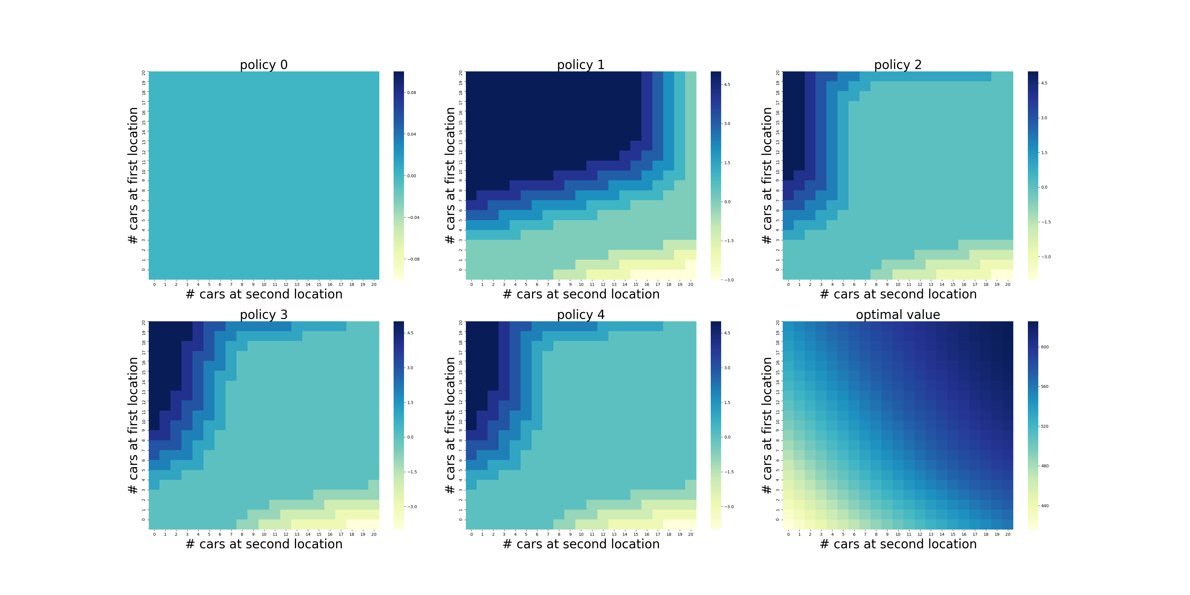
Results

The found optimal value function and optimal policy are illustrated below. The results match with book's illustrations.

In the optimal policy we see the reasonable tendency to balance number of cars in the locations. Because the rental request rate in the location 1 is higher we are more willing to move cars there and less willing to move it in other direction.

Advanced problem

The book has also modified version of the task.

To solve it we only need to take into account the new details when computing \(r(s, a, s')\). All the rest stay the same. Updated computation of the tensors is located at components_adv.py. The results are illustrated below.

Here we see how we adapt to the new environment. For example, we use the free ride to balance number of cars at the locations when previously it was too costly. We have also become very selective in the number of cars moved to pay for additional parking only in one location. The value function has become unlinear.

Relevant links

• Sutton and Barto book's site
• Other problem's implementation in Python